Turn Signals and Road Behavior
Detailed analysis of route segmentation for turn signal activation
The trajectory generated for the virtual QCar 2 was not used solely as a geometric navigation reference, but also as a basis for incorporating explicit road behavior, particularly turn signal activation. This decision was relevant because, within an autonomous driving system designed for an urban-like environment, it is not enough for the vehicle to follow a curve correctly or remain close to a target trajectory; it must also visually communicate its maneuvers when entering, leaving, or crossing intersections, when switching branches within the road network of the map, or when executing a clearly identifiable regulatory turn.
For this reason, once the global smoothed trajectory had been obtained through graph-based planning and PCHIP interpolation, an additional route segmentation process was carried out. This process consisted of determining which parts of the trajectory corresponded to maneuvers where the left turn signal should be activated and which parts corresponded to maneuvers where the right turn signal should be activated. This processing layer allowed the vehicle not only to navigate the map correctly, but also to do so with a signaling logic consistent with the road rules defined for the environment.
Example of generated trajectory from node 1 to node 30
As a planning example, a trajectory calculated between node 1 and node 30 is presented. The following figure shows the final route obtained for that path.
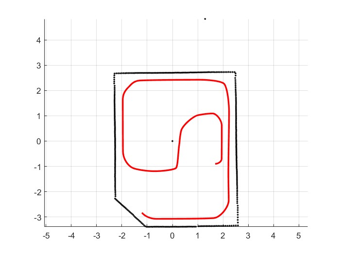
Figure. Global trajectory generated as a planning example between node 1 and node 30. The red curve represents the final smoothed trajectory that the virtual QCar 2 would follow, while the black dotted outline corresponds to the geometric reference frame of the environment.
In this figure, it can be observed that the trajectory covers an important portion of the circuit, passing through straight segments, wide curves, and a central area of higher geometric complexity. This confirms that the planning stage does not produce a simple linear connection between origin and destination, but rather a continuous route that is physically consistent with the topology of the map. From the control perspective, this red curve is the nominal reference that the vehicle would follow in the absence of external events such as signs, pedestrians, or obstacles.
However, for turn signal logic, it is not enough to know the overall shape of the trajectory. Although this curve is continuous, turn signaling must be decided based on the road-related meaning of certain path segments and not simply on the presence of curvature. As a result, it was necessary to build an additional logic capable of projecting traffic rules, originally defined over discrete graph nodes, onto the continuous trajectory that the vehicle actually follows.
General criterion for defining turn signal rules
The turn signal rules were not defined using a simplistic geometric criterion such as “if the curve goes left, then activate the left signal” or “if the path curves right, then activate the right signal.” That approach would have been too crude, because a smoothed trajectory may present local curvature for purely geometric reasons without that necessarily representing a road maneuver that should be announced with a turn signal.
For example, a vehicle may follow a smooth curve simply by following the natural shape of the lane, without changing branches or crossing an intersection. In that case, even though the trajectory is geometrically curved, from a road-behavior standpoint there is not necessarily a regulatory maneuver that requires signaling. In contrast, there are indeed transitions between graph nodes that represent explicit road decisions, such as:
- merging into a new branch of the map,
- crossing an intersection,
- leaving a main trajectory to take an exit,
- switching between an outer loop and an inner loop,
- completing an extended turn during which the turn signal should remain active over several consecutive subsegments.
For this reason, the rules were defined over the topology of the map, that is, over the discrete transitions between nodes that truly represent traffic maneuvers.
Traffic rules for turn signal activation
The rules defined for turn signal activation were the following.
Left turn signal rules
- 7 → 8
- 8 → 9
- 15 → AUX
- AUX → 24
- 17 → 6
- 23 → AUX
- AUX → 32
- 27 → 7
- 31 → AUX
- AUX → 45
- 44 → AUX
- AUX → 16
Right turn signal rules
- 9 → 41
- 13 → 46
- 15 → 45
- 17 → 18
- 23 → 16
- 26 → 27
- 27 → 28
- 31 → 25
- 39 → 40
- 40 → 41
- 41 → 42
- 44 → 32
- 45 → 3
Auxiliary node AUX
In these rules, the symbol AUX corresponds to node 48, located at the center of the main intersection on the map. This node is not part of the minimal original graph structure, but was introduced as an auxiliary node to improve the geometric and semantic representation of certain crossings, mainly the more complex left turns.
The importance of this node is considerable. If a left-turn crossing were represented directly between two extreme nodes, the resulting trajectory could appear too abrupt, unnatural, or even poorly representative of how a vehicle actually crosses an intersection. By forcing the trajectory to pass through the central auxiliary node, the curve develops more progressively and the section in which the turn signal remains active extends over the entire maneuver, rather than only at the exact instant of connection between two branches.
In other words, AUX = 48 simultaneously improves two aspects of the system:
- the geometry of the turn, by smoothing complex crossings,
- the road semantics of the signaling, by making the turn signal cover a more realistic maneuver.
Topological and road-related justification of the left-turn rules
7 → 8 and 8 → 9
These two transitions were classified as the same left turn signal maneuver because they represent a continuous merge in the upper part of the map. This was not treated as a punctual activation at a single vertex, but rather as an extended maneuver covering two consecutive subsegments. From a road-behavior perspective, this decision is more appropriate than turning the signal on and off at a single point, since the vehicle maintains a sustained change in orientation until it aligns with the next main segment of the circuit.
15 → AUX and AUX → 24
This case represents one of the most important left-turn crossings in the central intersection. The vehicle enters the intersection from one branch, passes through the center, and exits toward another branch with a clear left turn. Here, the auxiliary node is essential because it divides the maneuver into two phases: approach to the center and exit from the center toward the target branch. This allows the turn signal to remain active throughout the entire intersection traversal and not only at the exact instant of the crossing.
17 → 6
This transition was labeled as a left maneuver because, within the topological logic of the map, it represents a merge from an inner branch into another main branch. Although geometrically the connection may appear as a moderate curve, from a road perspective it implies leaving one trajectory to merge into another, which justifies turn signal activation.
23 → AUX and AUX → 32
This case is analogous to the crossing 15 → AUX → 24, but applied to another transition within the central intersection. Once again, the vehicle traverses a topological decision area where it not only changes orientation, but also changes branch within the road network. Splitting the maneuver into two segments around the AUX node allows the turn signal to remain active throughout the entire left-turn crossing.
27 → 7
This rule represents a merge from an inner trajectory toward the upper or outer part of the circuit. It is not simply a continuation along the same branch, but rather taking a different connection within the map, which is why it was interpreted as a left maneuver from the road-behavior standpoint.
31 → AUX and AUX → 45
This case corresponds to another left-turn crossing through the center of the intersection. As in the previous cases, the use of the auxiliary node avoids an abrupt transition between distant branches and distributes turn signal activation over a longer and more realistic portion of the trajectory.
44 → AUX and AUX → 16
This pair of rules describes another relevant left-turn crossing within the map. From node 44, the vehicle can enter the center of the intersection and exit toward another branch, describing a maneuver that is road-wise equivalent to a left turn. The use of AUX allows that maneuver to be captured with greater geometric fidelity.
Topological and road-related justification of the right-turn rules
9 → 41
This transition represents an exit from the upper part of the circuit toward an inner branch. Although the smoothed trajectory may describe this change continuously, from the graph topology this connection constitutes a concrete road decision: leaving the current trajectory and taking another branch. For that reason, it was marked as a right turn signal maneuver.
13 → 46
This connection corresponds to a lateral exit in the left side of the map, where the vehicle leaves the main vertical branch to enter an alternate connector. It is a short maneuver, but clearly significant from a regulatory standpoint.
15 → 45
This transition is especially interesting because it shares the same origin node as the maneuver 15 → AUX → 24, but represents a different exit. From node 15, the vehicle can choose between two different paths within the intersection: one associated with a left crossing and another associated with an exit to the right. This shows that turn signal logic does not depend on the isolated node, but on the specific transition between nodes.
17 → 18
This transition represents the vehicle entering a descending branch located on the right side of the map. The change in orientation and branch is clear enough to be interpreted as a right maneuver.
23 → 16
This case is the right-turn alternative to the left-turn crossing 23 → AUX → 32. From node 23, the vehicle can move toward different branches, and each of those exits has a different road meaning. The transition toward 16 was interpreted as a right maneuver.
26 → 27 and 27 → 28
These two consecutive transitions were grouped as a single extended right turn signal maneuver. The logic here is equivalent to that of the longer left maneuvers: keeping the signal active throughout the full development of the maneuver and not only at one of its vertices.
31 → 25
This connection represents another exit from a main branch toward a different trajectory. It was classified as right because the vehicle leaves its current flow in order to merge into another direction of circulation within the map.
39 → 40, 40 → 41, and 41 → 42
This set of three segments is one of the best examples of an extended maneuver. Instead of a punctual activation, the right turn signal was kept active across three consecutive subsegments, so that the entire branch change would be properly signaled. This demonstrates that the system is capable of representing long maneuvers as continuous road entities.
44 → 32
This case is the right-turn alternative to the left-turn crossing 44 → AUX → 16. From the same origin node, there are different road decisions, and therefore each transition must have its own turn signal logic. This reinforces the idea that the rules are defined over the directed graph and not only over local geometry.
45 → 3
Finally, this transition represents a connection from the lower central area toward another branch of the circuit. It was considered a right maneuver because the vehicle leaves the trajectory it was on and enters a new circulation branch.
Script to generate the turn signal segments
Once the rules over node pairs had been defined, it was necessary to build a procedure that translated them into actual segments over the smoothed trajectory. The script used for that purpose was the following:
%% =============================
% NODE → TRAJECTORY INDEX MAPPING
% =============================

num_nodes_path = length(pathNodes_corrected);
node_to_idx = zeros(num_nodes_path,1);

search_start = 1; % key: avoids ambiguities
AUX = 48;

for k = 1:num_nodes_path

    nodo_id = pathNodes_corrected(k);
    nodo_xy = nodes(nodo_id,:);

    min_dist = inf;
    best_idx = search_start;

    for i = search_start:length(path_x_smooth)

        dx = path_x_smooth(i) - nodo_xy(1);
        dy = path_y_smooth(i) - nodo_xy(2);
        d = dx^2 + dy^2; % no sqrt (faster)

        if d < min_dist
            min_dist = d;
            best_idx = i;
        end
    end

    node_to_idx(k) = best_idx;
    search_start = best_idx; % search only forward
end

%% =============================
% DEFINE YOUR RULES
% =============================

der = [9 41; 13 46; 15 45; 17 18; 23 16; 26 27; 27 28;
       31 25; 39 40; 40 41; 41 42; 44 32; 45 3];

izq = [7 8; 8 9; 15 AUX; AUX 24; 17 6; 23 AUX; AUX 32; 27 7; 31 AUX; AUX 45; 44 AUX; AUX 16];

%% =============================
% CREATE SEGMENTS
% =============================

segmentos_izq = [];
segmentos_der = [];

for k = 1:length(pathNodes_corrected)-1

    n1 = pathNodes_corrected(k);
    n2 = pathNodes_corrected(k+1);

    idx1 = node_to_idx(k);
    idx2 = node_to_idx(k+1);

    segmento = [min(idx1,idx2), max(idx1,idx2)];

    % Check whether this segment is in your rules

    if any(all(izq == [n1 n2],2))
        segmentos_izq = [segmentos_izq; segmento];
    end

    if any(all(der == [n1 n2],2))
        segmentos_der = [segmentos_der; segmento];
    end

end

%% =============================
% (OPTIONAL) MERGE CONTIGUOUS SEGMENTS
% =============================

merge_segments = @(seg) ...
    cell2mat(arrayfun(@(i) ...
    [seg(i,1), seg(find(seg(:,1)==seg(i,2),1,'first'),2)], ...
    1:size(seg,1)-1, 'UniformOutput', false)');

%% =============================
% SAVE
% =============================

save('segmentos_direccionales.mat', 'segmentos_izq', 'segmentos_der');

%% =============================
% VISUALIZATION
% =============================

figure; hold on; grid on; axis equal;

h_traj = plot(path_x_smooth, path_y_smooth, 'k');

% LEFT (green)
h_izq = [];
for i = 1:size(segmentos_izq,1)
    idx = segmentos_izq(i,1):segmentos_izq(i,2);
    h_izq = plot(path_x_smooth(idx), path_y_smooth(idx), 'g', 'LineWidth', 3);
end

% RIGHT (red)
h_der = [];
for i = 1:size(segmentos_der,1)
    idx = segmentos_der(i,1):segmentos_der(i,2);
    h_der = plot(path_x_smooth(idx), path_y_smooth(idx), 'r', 'LineWidth', 3);
end

legend([h_traj, h_izq, h_der], {'Path', 'left turn signal', 'right turn signal'});
Detailed explanation of the script
1. Mapping nodes to indices of the smoothed trajectory
The trajectory that the vehicle actually follows is not composed of nodes, but of thousands of interpolated points stored in path_x_smooth and path_y_smooth. For that reason, the first part of the script seeks to associate each node of the corrected route with a real index on the continuous trajectory.
If the continuous trajectory is denoted by:
\[\mathcal{P} = {(x_1,y_1), (x_2,y_2), \dots, (x_M,y_M)}\]and each corrected node by:
\[v_k = (x_k^{node}, y_k^{node}),\]then the index associated with each node is computed as:
\[i_k^\star = \arg\min_{i \ge i_{k-1}^\star} \left[(x_i - x_k^{node})^2 + (y_i - y_k^{node})^2\right]\]Using squared distance avoids the square root and makes the computation more efficient. In addition, the variable search_start forces the search always to move forward, which avoids ambiguities in trajectories where the path comes close to previously traversed areas.
2. Applying rules over transitions between nodes
Once the node_to_idx array has been obtained, the script traverses the sequence pathNodes_corrected by taking consecutive pairs ((n_1,n_2)). For each transition, it checks whether that pair belongs to the izq list or to the der list.
If the pair belongs to izq, a left segment is created.
If it belongs to der, a right segment is created.
In this way, the algorithm transforms a discrete topological rule into an actual interval over the continuous trajectory.
3. Segment construction
Each section is represented as an interval of indices:
\[I_k = [\min(i_k^\star, i_{k+1}^\star),\ \max(i_k^\star, i_{k+1}^\star)]\]This means that the turn signal is not activated at a single point, but over an entire continuous region of the trajectory. This decision is correct from the vehicle behavior standpoint, because a turn signal must remain active throughout the full development of the maneuver and not only when crossing one graph vertex.
4. Optional merging of contiguous segments
The script proposes an optional merge_segments function to merge contiguous segments. Although this function is not strictly necessary for basic visualization, it may be useful if one wants to simplify the representation and group long maneuvers into a single continuous region.
5. Saving and visualization
The resulting segments are saved into the segmentos_direccionales.mat file, which makes it possible to reuse them later in other system modules, for example in the light controller block. Finally, the script generates a figure where:
- the full trajectory appears in black,
- the left-turn-signal segments appear in green,
- the right-turn-signal segments appear in red.
Figure of turn signal segmentation for the node 1 to node 30 example
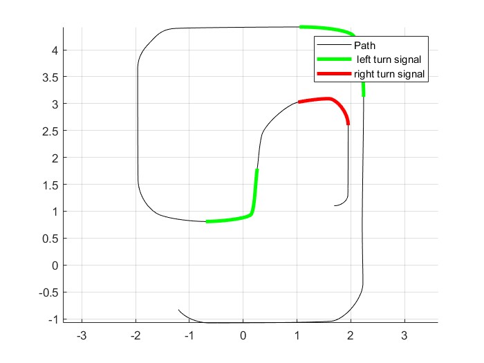
Figure. Segmentation of the trajectory corresponding to the planning example between node 1 and node 30. The complete route is shown in black, the segments where the left turn signal must be activated appear in green, and the segments where the right turn signal must be activated appear in red.
Interpretation of the result
The segmentation figure demonstrates that turn signal activation was not defined arbitrarily or solely from the visual curvature of the trajectory. Each colored segment corresponds to a graph transition whose road-related interpretation had been previously encoded. This makes it possible for the vehicle to combine two different levels of intelligence within the system:
- geometric tracking, based on the smoothed trajectory,
- semantic road behavior, based on topological rules over nodes.
The green segments represent maneuvers in which the vehicle must announce a left turn or merge, while the red segments correspond to equivalent maneuvers to the right. The fact that these regions are located exactly over specific parts of the trajectory confirms that the mapping between nodes and the interpolated curve was correct.
In addition, the use of the auxiliary node AUX = 48 is particularly valuable in complex intersections, since it makes it possible to model left turns as a continuous sequence rather than as an abrupt transition between extreme nodes. Consequently, the turn signal remains active over a portion of trajectory that is more representative of the actual maneuver.