Global Trajectory Planning
2. Global trajectory planning through directed graphs, QLabs map coordinates, and road-related penalties
The vehicle reference trajectory was not drawn manually. Instead, it was constructed from a topological representation of the competition circuit, obtained directly from the QLabs map. To do so, strategic points were selected along the road network of the virtual environment, and each one was assigned Cartesian coordinates $(x,y)$. These points were converted into nodes of a directed graph, while the physically traversable connections between them were modeled as edges.
From the perspective of navigation engineering, this methodology makes it possible to convert a continuous mobility problem into a discrete network optimization problem. Instead of continuously asking “where should the vehicle move on the plane,” the vehicle first solves “through which sequence of nodes should it pass in order to reach the destination with the minimum possible cost.” That discrete sequence is then smoothed to generate a continuous trajectory that can be physically followed by the controller.
2.1 Modeling the set of nodes
If
\[V = \{v_1, v_2, \dots, v_N\}\]denotes the set of nodes, then each node is defined as:
\[v_i = (x_i, y_i)\]In this project, 47 nodes were used, that is:
\[N = 47\]The node matrix was:
nodes = [
   -1.2050  -0.83
   -0.63    -1.076
   0.533    -1.071
   1.626    -1.045
   2.225    -0.337
   2.212    0.756
   2.238    3.125
   2.029    4.279
   1.047    4.425
   -1.274   4.397
   -1.716   4.156
   -1.963   3.630
   -1.956   1.596
   -1.541   0.927
   -0.696   0.809
   0.945    0.815
   1.711    0.802
   1.945    0.138
   1.945    -0.376
   1.704    -0.714
   0.799    -0.811
   0.357    -0.550
   0.260    0.068
   0.260    1.791
   0.344    2.409
   1.021    3.027
   1.587    3.092
   1.951    2.598
   1.945    1.303
   1.691    1.102
   1.001    1.076
   -0.696   1.063
   -1.534   1.252
   -1.690   1.843
   -1.696   3.559
   -1.521   3.974
   -1.177   4.150
   0.331    4.158
   0.520    4.106
   0.767    3.931
   0.897    3.638
   0.767    3.170
   0.240    2.675
   -0.007   1.759
   0.006    0.068
   -1.937   0.4
   -1.696   -0.399
];
These nodes were extracted from the QLabs map and placed at key positions of the circuit: curvature changes, entrances and exits of intersections, connections between the outer and inner loops, as well as zones relevant for turning maneuvers and lane transitions.
Each node represents a geometrically relevant position within the road network. For example, if a node appears at the entrance of an intersection, its function is not merely to “mark a point,” but to divide the map into navigable segments with a logical flow for the vehicle. This allows planning to depend not only on the visual shape of the circuit, but also on its functional structure.
2.2 Modeling the set of edges
A directed edge
\[e_{ij} = (v_i, v_j)\]indicates that the vehicle can move from node $i$ to node $j$. The complete graph is therefore defined as:
\[G = (V, E, W)\]where $E$ is the set of edges and $W$ is the set of associated weights.
edges = [
   1 2;
   2 3;
   3 4;
   4 5;
   5 6;
   6 7;
   7 8;
   8 9;
   9 10;
   10 11;
   11 12;
   12 13;
   13 14;
   13 46;
   14 15;
   15 16;
   15 45;
   15 24;
   16 17;
   17 18;
   17 6;
   18 19;
   19 20;
   20 21;
   21 22;
   22 23;
   23 16;
   23 24;
   23 32;
   24 25;
   25 26;
   26 27;
   27 28;
   27 8;
   28 29;
   29 30;
   30 31;
   31 32;
   31 24;
   31 45;
   32 33;
   33 34;
   34 35;
   35 36;
   36 37;
   37 38;
   38 39;
   39 40;
   40 41;
   41 42;
   41 27;
   42 43;
   43 44;
   44 45;
   44 32;
   44 16;
   45 3;
   46 47;
   47 1;
];
The use of a directed graph is essential, since not all circuit connections are equivalent or symmetric. This forces the planner to respect the traffic flow logic of the environment and prevents physically infeasible routes or routes that go against the expected direction of travel.
2.3 Geometric distance between nodes
For each edge $(i,j)$, the Euclidean distance between the origin node and the destination node is first computed:
\[d_{ij} = \sqrt{(x_j - x_i)^2 + (y_j - y_i)^2}\]In code:
numEdges = size(edges,1);
weights = zeros(numEdges,1);

for k = 1:numEdges
    i = edges(k,1);
    j = edges(k,2);

    dx = nodes(j,1) - nodes(i,1);
    dy = nodes(j,2) - nodes(i,2);

    dist = sqrt(dx^2 + dy^2);

    weights(k) = dist + penalty(k);
end
This distance represents the purely geometric cost of traveling between two consecutive nodes. If planning depended only on this term, the vehicle would always choose the shortest total route. However, in a road environment, that does not always lead to the best trajectory from an operational standpoint.
2.4 Penalty for road-related complexity
One of the most important decisions of the project was not to select the trajectory based solely on geometric length. In an autonomous driving system, the shortest route is not always the most convenient one, since certain segments of the map imply greater operational complexity due to the presence of road elements such as traffic lights, stop signs, crosswalks, roundabouts, or yield signs. For this reason, each edge of the graph was assigned an additional penalty according to the elements present along that segment.
The penalty table used was the following:
| Road element | Penalty |
|---|---|
| Traffic light | 3 |
| Stop signal | 4 |
| Crosswalk | 2 |
| Round signal | 1 |
| Yield signal | 1 |
In this way, if an edge connects two nodes and more than one road element exists along that segment, the total penalty of that edge is obtained by summing the individual contributions of all the elements present. Mathematically, the penalty associated with the edge connecting node $i$ to node $j$ is defined as:
\[p_{ij} = 3,n_{tl,ij} + 4,n_{stop,ij} + 2,n_{cw,ij} + 1,n_{round,ij} + 1,n_{yield,ij}\]where:
- $n_{tl,ij}$: number of traffic lights on the segment
- $n_{stop,ij}$: number of stop signs
- $n_{cw,ij}$: number of crosswalks
- $n_{round,ij}$: number of roundabout-related elements
- $n_{yield,ij}$: number of yield signs
Therefore, the total weight of each edge does not depend only on its geometric length, but on the sum of its distance and its road-related penalty:
\[w_{ij} = d_{ij} + p_{ij}\]where $d_{ij}$ is the Euclidean distance between nodes $i$ and $j$, computed as:
\[d_{ij} = \sqrt{(x_j - x_i)^2 + (y_j - y_i)^2}\]This formulation allows the planning algorithm to prefer trajectories that are not only shorter, but also more convenient from an operational point of view.
Example of penalty application
If between two nodes on the map, for example between node $n$ and node $m$, there is a crosswalk and a stop signal, then the total penalty for that segment is calculated as:
\[p_{nm} = 2 + 4 = 6\]and therefore the final weight of the edge becomes:
\[w_{nm} = d_{nm} + 6\]Similarly, if a segment contains a traffic light and a yield sign, the penalty would be:
\[p_{ij} = 3 + 1 = 4\]This criterion transforms the planning problem into an optimization problem over a weighted map, where the vehicle seeks the route with the minimum total cost and not simply the one with the minimum distance.
2.5 Penalty vector used
penalty = zeros(size(edges,1),1);

penalty(1) = 0;
penalty(2) = 0;
penalty(3) = 0;
penalty(4) = 0;
penalty(5) = 4;
penalty(6) = 1;
penalty(7) = 1;
penalty(8) = 0;
penalty(9) = 0;
penalty(10) = 0;
penalty(11) = 0;
penalty(12) = 0;
penalty(13) = 0;
penalty(14) = 0;
penalty(15) = 0;
penalty(16) = 7;
penalty(17) = 7;
penalty(18) = 7;
penalty(19) = 2;
penalty(20) = 0;
penalty(21) = 0;
penalty(22) = 0;
penalty(23) = 0;
penalty(24) = 0;
penalty(25) = 0;
penalty(26) = 0;
penalty(27) = 7;
penalty(28) = 7;
penalty(29) = 7;
penalty(30) = 0;
penalty(31) = 0;
penalty(32) = 2;
penalty(33) = 0;
penalty(34) = 0;
penalty(35) = 2;
penalty(36) = 0;
penalty(37) = 0;
penalty(38) = 7;
penalty(39) = 7;
penalty(40) = 7;
penalty(41) = 0;
penalty(42) = 0;
penalty(43) = 4;
penalty(44) = 0;
penalty(45) = 0;
penalty(46) = 2;
penalty(47) = 2;
penalty(48) = 0;
penalty(49) = 0;
penalty(50) = 0;
penalty(51) = 0;
penalty(52) = 0;
penalty(53) = 0;
penalty(54) = 7;
penalty(55) = 7;
penalty(56) = 7;
penalty(57) = 0;
penalty(58) = 2;
penalty(59) = 0;
This vector represents the practical translation of the road evaluation carried out over the different segments of the map. In engineering terms, what was done was to assign each edge of the graph an additional cost derived from the road context associated with it. This means that the map was not treated as a simple collection of geometric distances, but rather as a network of paths with different levels of operational complexity.
2.6 Obtaining the optimal route
The optimal route is obtained by solving the problem:
\[P^\star = \arg\min_{P \in \mathcal{P}(s,g)} \sum_{(i,j)\in P} w_{ij}\]where $s$ is the initial node and $g$ is the goal node.
G = digraph(edges(:,1), edges(:,2), weights);

startNode = 1;
goalNode = 44;

[pathNodes, totalCost] = shortestpath(G, startNode, goalNode);
Here, the vehicle starts at node 1 and heads toward node 44. The variable pathNodes contains the discrete sequence of nodes that minimizes the total cost. The variable totalCost represents the accumulated value of that objective function.
2.7 Geometric correction of critical crossings
Although the resulting discrete route is optimal in terms of the graph, some transitions at intersections may be geometrically poor. To solve this, an auxiliary central node was defined:
centro_interseccion = [0.144, 0.939];

casos_criticos = [23, 32;
                  15, 24;
                  44, 16;
                  31, 45];
and it is inserted whenever a critical connection appears:
pathNodes_corrected = [];

for k = 1:length(pathNodes)-1
    nodo_actual = pathNodes(k);
    nodo_siguiente = pathNodes(k+1);

    pathNodes_corrected = [pathNodes_corrected, nodo_actual];

    es_critico = any(all(casos_criticos == [nodo_actual, nodo_siguiente], 2));

    if es_critico
        nodes(end+1, :) = centro_interseccion;
        pathNodes_corrected = [pathNodes_corrected, size(nodes,1)];
    end
end
pathNodes_corrected = [pathNodes_corrected, pathNodes(end)];
This correction does not change the global logic of the shortest path, but it does improve its local geometric shape. The auxiliary node acts as an additional support point in areas where a direct turn between extreme nodes would produce an unnatural curve for the vehicle.
2.8 Trajectory smoothing using PCHIP
Once the discrete sequence has been corrected, a continuous trajectory is generated:
path_x_final = nodes(pathNodes_corrected, 1);
path_y_final = nodes(pathNodes_corrected, 2);

t_new = 1:length(path_x_final);
tq_new = linspace(1, length(path_x_final), 1761);

path_x_smooth = interp1(t_new, path_x_final, tq_new, 'pchip');
path_y_smooth = interp1(t_new, path_y_final, tq_new, 'pchip');
Mathematically:
\[x_s(\tau) = \operatorname{PCHIP}(t_k, x_k), \qquad y_s(\tau) = \operatorname{PCHIP}(t_k, y_k)\]where $(x_k, y_k)$ are the corrected discrete points and $\tau$ is the continuous interpolation parameter.
The use of PCHIP is especially appropriate because it preserves the local shape of the trajectory better and avoids artificial oscillations. This is important for the autonomous vehicle, since a reference that is too wavy or has abrupt curvature changes may make stable tracking more difficult for the controller.
2.9 Final trajectory visualization
load distance_new_qcar2.mat;
load angles_new_qcar2.mat;

range_qcar2 = distance_new_qcar2(:,end);
angles_qcar2 = angles_new_qcar2(:,end);

qcar2_lidar_to_map_rotation = -1.5 * pi/180;
cal_pos = [0, 2, 0];

figure(1)
hold on;

polar(-angles_qcar2-qcar2_lidar_to_map_rotation, range_qcar2,'k.');

plot(path_x_smooth - cal_pos(1), ...
     path_y_smooth - cal_pos(2), ...
     'r', 'LineWidth', 2);

axis equal
grid on
hold off;

path_x_dijkstra  = path_x_smooth(:);
path_y_dijkstra  = path_y_smooth(:);
Figure of the base map with graph nodes
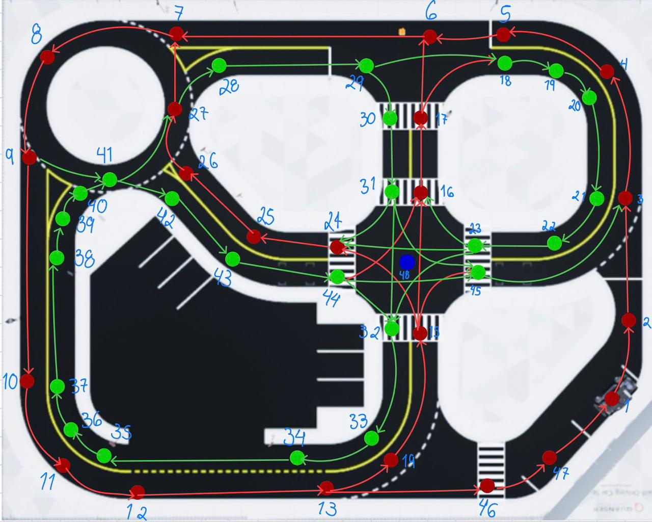
Technical description of the figure. The figure shows the competition map used to construct the planning system graph. Numbered nodes were placed over the circuit at key positions of the environment: curvature changes, entrances and exits of intersections, connections between the outer and inner loops, and zones near relevant road events. From these coordinates, the topological structure of the problem was constructed.
Figure of the generated global trajectory
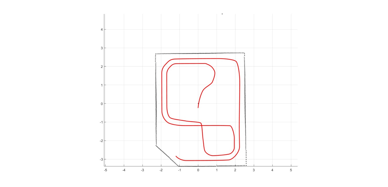
Technical description of the figure. The red line represents the final global trajectory that the virtual QCar 2 would follow within the simulation environment. This trajectory was obtained by solving an optimization problem over the directed graph of the map and then smoothing the discrete route through PCHIP interpolation, in order to generate a continuous reference that is physically more suitable for vehicle tracking. The black dotted line corresponds to the spatial frame of the environment used as the calibration reference. It is important to note that this trajectory is presented only as an example of planning between node 1 and node 44.
Interpretation of this section within the complete system
Global planning constitutes the backbone of the nominal behavior of the vehicle. All other modules of the system — object detection, signal logic, depth estimation, turn signals, and obstacle avoidance — are built on top of this trajectory reference. If the planning were not consistent, stable, or geometrically reasonable, the rest of the pipeline would operate on a defective foundation.
For this reason, this section does not merely define a route, but rather constructs a structured navigation space where each segment has both geometric and operational meaning. The combination of coordinates extracted from the map, directed edges, road penalties, geometric correction, and final interpolation makes it possible to obtain a trajectory that not only connects an origin and a destination, but is also appropriate to be followed by the vehicle in a simulated urban environment.