Visual Perception and Simulink-Python Communication

3. Training and validation of the object detection model for Quanser City

A fundamental part of the self-driving system was the development of the visual perception module. In the context of the competition, it was not enough for the vehicle to follow a predefined trajectory; it also had to be capable of identifying relevant elements in the environment, such as cones, traffic signs, and traffic lights, in order to modify its behavior in real time. For this reason, a neural network specifically oriented to the Quanser City scenario was trained.

The selected model was a variant of YOLOv8, trained in Google Colab with GPU support and later exported to the ONNX format in order to facilitate its integration into the Simulink stack. This decision was important because it allowed the training problem to be separated from the deployment problem. Training was carried out in a flexible GPU-accelerated environment, while the final execution was integrated into the vehicle architecture through an external Python service.

3.1 Objective of the perception model

The purpose of the model was to transform RGB images from the virtual environment into a structured representation of detected objects. If an image captured by the vehicle is denoted as:

\[I \in \mathbb{R}^{H \times W \times 3}\]

then the goal of the detector is to estimate a set of objects:

\[\mathcal{D} = \{d_1, d_2, \dots, d_n\}\]

where each detection is described by a class, a confidence value, and a bounding box:

\[d_i = (c_i,\ \rho_i,\ x_{1,i},\ y_{1,i},\ x_{2,i},\ y_{2,i})\]

Here:

• $c_i$ is the detected class,
• $\rho_i$ is the probability or confidence of the model,
• $(x_{1,i}, y_{1,i})$ and $(x_{2,i}, y_{2,i})$ are the bounding box coordinates.

This structure constitutes the basis of the rest of the pipeline, since it will later be enriched with depth information and used by the vehicle decision-making logic.

3.2 Verification of the computing environment

Before training the model, it was necessary to verify that the Colab environment had access to a GPU. The following code was used for that purpose:

import torch
print(torch.cuda.is_available())  # Should print True
print(torch.cuda.device_count())  # Should print 1 or more

This verification is important because training a convolutional detector over multiple epochs and moderate-resolution images requires significant computational resources. The use of a GPU drastically reduces training time and makes it feasible to iterate on the model within a practical workflow.

3.3 Installation of the Ultralytics library and environment check

!pip install ultralytics

import ultralytics
ultralytics.checks()

In this part, the ultralytics library is installed, which provides the YOLOv8 implementation used in the project. The call to ultralytics.checks() verifies that the execution environment is consistent and that the required dependencies are properly configured. This includes validations related to PyTorch, CUDA, memory, and the general execution environment.

3.4 Dataset loading and preparation

from google.colab import files
uploaded = files.upload()

!unzip detection_2025.v8i.yolov8.zip

!ls
!ls valid
!ls test
!ls train

At this stage, the training dataset is uploaded and extracted. The dataset organization into train, valid, and test folders follows a standard supervised learning methodology:

• train: set used to fit the model parameters
• valid: set used to monitor performance during training
• test: set used to evaluate the final behavior of the model on unseen data

This separation helps reduce the risk of overfitting and provides a more solid basis for evaluating whether the detector truly generalizes to new images from the environment.

3.5 Model training

from ultralytics import YOLO

model = YOLO("yolov8s.pt")

model.train(
    data="data.yaml",
    epochs=150,
    imgsz=640,
    batch=32
)

Here, the base model is defined using the pretrained checkpoint yolov8s.pt. The choice of this variant reflects a trade-off between representational capacity and computational cost. A model that is too small might fail to detect traffic signs or small objects properly, while a model that is too large could be more expensive to train and less practical to deploy.

The main training parameters were:

• epochs=150: number of optimization epochs
• imgsz=640: input image size
• batch=32: batch size

From a mathematical perspective, training seeks to solve a loss minimization problem:

\[\theta^\star = \arg\min_{\theta} \mathcal{L}(\theta)\]

where $\theta$ represents the model parameters and $\mathcal{L}$ the total detector loss function. In YOLO, this loss typically combines classification errors, bounding box localization errors, and detection confidence errors.

The data.yaml file contains the dataset definition, including classes and paths to the corresponding subsets. This is essential for the model to understand the structure of the classification/detection problem it must learn.

3.6 Export to ONNX

model.export(format="onnx", opset=12)

Once the model was trained, it was exported to ONNX format. This decision was very important from the integration standpoint. Although training was carried out in Colab, inference later had to be executed within an architecture connected to Simulink. ONNX provides an interoperable format that facilitates deployment of the model outside the original training environment.

In other words, the full workflow was:

\[\text{Training in Colab} \rightarrow \text{Model } .pt \rightarrow \text{Export to ONNX} \rightarrow \text{Inference connected to Simulink}\]

3.7 Quantitative validation of the model

model = YOLO("runs/detect/train/weights/best.pt")
metrics = model.val(data="data.yaml")
print("mAP@50:", metrics.box.map50)
print("mAP@50-95:", metrics.box.map)
print("Precision:", metrics.box.mp)
print("Recall:", metrics.box.mr)

After training, standard metrics were computed to evaluate detector performance. If these metrics are denoted in a general form as:

• $mAP_{50}$: mean average precision with IoU = 0.50
• $mAP_{50{-}95}$: mean average precision over multiple IoU thresholds
• $P$: precision
• $R$: recall

then the perception module can be quantitatively evaluated through:

\[P = \frac{TP}{TP + FP}\] \[R = \frac{TP}{TP + FN}\]

where:

• $TP$: true positives
• $FP$: false positives
• $FN$: false negatives

The metric $mAP_{50}$ evaluates mean precision when a detection is considered correct if its intersection over union exceeds 0.50. The metric $mAP_{50{-}95}$ is more demanding because it averages performance over multiple IoU thresholds, providing a more robust evaluation of detector quality.

3.8 Qualitative test of the exported model

from ultralytics import YOLO
from IPython.display import display
from PIL import Image

model = YOLO("/content/best.onnx")

image_path = "/content/test/images/front_1743683028_9531693_jpg.rf.56133166b031d652d8dcacb3a1fc7015.jpg"

results = model(image_path)
results[0].save(filename="/content/deteccion.jpg")

display(Image.open("/content/deteccion.jpg"))

This test made it possible to verify that the model exported to ONNX continued to function correctly before integrating it with Simulink. This step is important because a model may behave properly in its original training format and still show unexpected differences after conversion to another format. Validating the exported model reduces that risk and provides confidence in the deployment process.

---

4. Bidirectional communication between Simulink and Python

Once the model was trained, it was necessary to integrate it into the self-driving pipeline. To accomplish this, a Python script was developed to communicate with Simulink through TCP sockets. The system is bidirectional: Simulink sends frames to the script, and the script returns a structured list of detections.

The importance of this module lies in the fact that it serves as a bridge between two complementary environments:

• Simulink, which is used as the core of the control and decision system
• Python, which is used as the inference environment for the ONNX model

In this way, the architecture takes advantage of the strengths of both environments without losing modularity.

4.1 Initial service configuration

import socket
import numpy as np
import cv2
import threading

HOST = "localhost"
PORT = 18002

frame_size = 640*480*3
latest_frame = None
running = True

s = socket.socket()
s.bind((HOST, PORT))
s.listen(1)

print("Waiting for connection...")
conn, addr = s.accept()
print("Connected from:", addr)

Here, the frame size is defined as:

\[N_{bytes} = 640 \times 480 \times 3\]

which corresponds to an RGB image of resolution 640 by 480. The main socket is responsible for receiving from Simulink a continuous stream of bytes corresponding to each frame.

The variable latest_frame is used as a shared buffer between threads, while running acts as a global execution flag.

4.2 Creation of the return channel

send_socket = socket.socket()
send_socket.bind(("localhost", 18001))
send_socket.listen(1)

print("Waiting for Simulink return connection...")
conn_send, addr_send = send_socket.accept()
print("Simulink connected for return:", addr_send)

Here, a second independent channel is created, dedicated to returning results to Simulink. This separation between input and output channels simplifies the communication architecture and avoids ambiguities in the data flow.

In system terms, the structure becomes:

\[\text{Simulink} \xrightarrow[\text{frames}]{18002} \text{Python} \xrightarrow[\text{detections}]{18001} \text{Simulink}\]

4.3 Loading the inference model

print("Importing YOLO...")
from ultralytics import YOLO

print("Loading model...")
model = YOLO(r"C:\Users\desqu\OneDrive\Desktop\decimo semestre\sins autonomos\best2.onnx", task="detect")
print("Model loaded")

At this stage, the previously exported ONNX model is loaded. The instruction task="detect" explicitly states that the model will be used for object detection tasks. Once loaded, the model can be applied to every frame received from Simulink.

4.4 Frame reception thread

def receive_frames():
    global latest_frame, running

    while running:

        data = b''

        while len(data) < frame_size:
            packet = conn.recv(frame_size - len(data))
            if not packet:
                running = False
                return
            data += packet

        frame = np.frombuffer(data, dtype=np.uint8)
        frame = frame.reshape((480,640,3), order='F')
        frame = cv2.cvtColor(frame, cv2.COLOR_RGB2BGR)

        latest_frame = frame

This thread reconstructs each image from the received byte stream. There are two particularly important technical details here.

The first is the accumulation of bytes until the full expected frame size is reached. This prevents incomplete images from being processed.

The second is the use of:

order='F'

when reshaping the array. This is crucial because MATLAB/Simulink uses column-major storage order, while NumPy usually assumes row-major order. By using order='F', the frame is reconstructed respecting the way Simulink sent it, thus avoiding distortions or incorrect image reordering.

Afterward, the frame is converted from RGB to BGR for compatibility with OpenCV and the visualization routine.

4.5 Inference and result return thread

def inference_loop():
    global latest_frame, running

    while running:

        if latest_frame is None:
            continue

        frame = latest_frame.copy()

        results = model(frame, verbose=False)

        annotated = results[0].plot()

        MAX_DET = 10
        output = np.zeros((MAX_DET, 6), dtype=np.float32)

        boxes = results[0].boxes

        if boxes is not None:

            for i in range(min(len(boxes), MAX_DET)):

                cls = int(boxes.cls[i].item())
                conf = float(boxes.conf[i].item())
                x1, y1, x2, y2 = boxes.xyxy[i].cpu().numpy()

                output[i] = [cls, conf, x1, y1, x2, y2]

        data_bytes = output.flatten().tobytes()
        conn_send.sendall(data_bytes)
        print("Sending bytes:", len(data_bytes))

        cv2.imshow("detection", annotated)

        if cv2.waitKey(1) == 27:
            running = False
            break

This thread takes the most recent frame and runs inference on it. The detector output is converted into a fixed structure with capacity for up to 10 detections per frame:

\[\mathbf{d}*i = \begin{bmatrix} c_i \ \rho_i \ x*{1,i} \ y_{1,i} \ x_{2,i} \ y_{2,i} \end{bmatrix}\]

Each row of the output matrix represents a detection, and the complete matrix has dimensions:

\[10 \times 6\]

This design is important because it imposes a stable communication interface between Python and Simulink. Even when a frame contains fewer than 10 detections, the output always preserves the same structure, which greatly simplifies its subsequent processing within the model.

4.6 Concurrent execution

t1 = threading.Thread(target=receive_frames)
t2 = threading.Thread(target=inference_loop)

t1.start()
t2.start()

t1.join()
t2.join()

conn.close()
cv2.destroyAllWindows()

Execution is divided into two threads:

• t1: continuous image reception
• t2: continuous inference and result return

This concurrent structure makes it possible to decouple frame arrival from the execution time of the neural network. Instead of blocking the entire system while a frame is being processed, the module maintains a more fluid architecture closer to the behavior expected in real time.

Role of this section within the complete system

This section represents the perception layer of the self-driving system. The detector training provides the ability to recognize relevant objects in the environment, while the Simulink–Python communication makes it possible to integrate that capability into the vehicle architecture.

Taken together, this module transforms a raw image of the environment into a structured set of detections that will later be used by the depth estimation and decision-making functions. Therefore, it acts as the entry point of the system’s visual knowledge and constitutes an essential component that enables the vehicle to stop being a simple trajectory follower and become an agent capable of interpreting the environment in which it operates.

Analysis of the trained detection model performance

The metrics obtained during the validation stage show that the detection model achieved solid performance suitable for its integration into the autonomous driving pipeline. In the global evaluation over 504 images and 968 instances, the model obtained a precision of 0.9119, a recall of 0.9338, an mAP@50 of 0.9605, and an mAP@50-95 of 0.7938. These results indicate that the detector not only correctly identifies most of the objects present in the environment, but also maintains high quality in the localization of the bounding boxes. From an engineering perspective, these values are consistent with a reliable detector for perception tasks in a controlled environment such as Quanser City, especially considering that the system does not rely solely on visual classification, but also on depth information and subsequent decision logic.

The value of mAP@50 = 0.9605 indicates that, under a relatively flexible intersection-over-union criterion, the model is capable of correctly detecting almost all relevant objects in the environment. This means that for the practical self-driving problem in simulation, where the main interest is to recognize traffic signs, traffic lights, pedestrians, and cones with sufficient anticipation, the model offers a very high detection rate. On the other hand, the value of mAP@50-95 = 0.7938 shows that, when greater geometric precision is required in the overlap of the boxes, performance decreases, but remains in a good range. This difference between the two metrics is entirely expected, and its interpretation is important: the model recognizes the presence of objects very well, although the exact delineation of their contours still presents moderate variation when the IoU criterion becomes stricter.

The class-wise analysis also helps to better understand the behavior of the model. The categories with the best performance were yield, red, round, stop, and yellow, all with mAP@50 values above 0.97 or very close to it. This suggests that road-related signaling elements and traffic lights were learned in a particularly robust way, which is excellent news for the proposed architecture, since these objects precisely constitute the basis of the vehicle’s traffic-rule logic. In particular, the yield class achieved an mAP@50 of 0.987 and an mAP@50-95 of 0.828, showing very consistent recognition both in terms of presence and localization. Likewise, the red class obtained an mAP@50 of 0.981 and an mAP@50-95 of 0.873, reflecting especially strong detection of the red light, which is critical for system safety.

The green class showed interesting behavior: it reached a recall of 1.0, which means that the model was capable of recovering all the examples present during validation, although with a precision of 0.861, lower than that of the other classes. This suggests that the detector was highly sensitive to the presence of the green traffic light, but produced some additional false positives. From a functional point of view, this can be interpreted as a conservative tendency not to miss true green-light examples, although still with some confusion in certain cases. In contrast, the yellow class showed a precision of 0.969 and a recall of 0.957, indicating a very good balance between correct detection and a low false alarm rate.

The class with relatively weaker performance was person, with a precision of 0.831, a recall of 0.750, an mAP@50 of 0.898, and an mAP@50-95 of 0.658. Although it is still a useful result, it clearly marks pedestrian detection as the least robust point of the model compared with signs and traffic lights. This has a reasonable explanation: in general, the person class presents more variability in pose, apparent size, orientation, and partial occlusion than a rigid sign or a traffic light. In addition, within the simulation environment, the pedestrian may occupy a relatively small portion of the field of view depending on its distance from the vehicle. Precisely for this reason, it was appropriate to reinforce the architecture with an additional safety function based on depth, instead of depending exclusively on visual classification of pedestrians.

From a temporal perspective, the validation report also shows very favorable inference performance. The model presented approximately 1.3 ms of preprocessing, 6.9 ms of inference, and 1.3 ms of postprocessing per image. This corresponds to a total time close to 9.5 ms per frame, which theoretically amounts to a processing rate of more than 100 images per second on the Tesla T4 GPU used during validation. Although this value should not be interpreted as identical to the final performance within the complete system — since the real implementation also involves image transfer, sockets, Simulink, and additional logic — it does show that the detector by itself has sufficiently low latency to be incorporated into a near real-time pipeline.

Interpretation of the training and validation curves

The training plots show behavior consistent with healthy model convergence. In the upper part, the training losses train/box_loss, train/cls_loss, and train/dfl_loss decrease steadily throughout the epochs. The reduction in box_loss indicates that the network learned to fit the bounding boxes around the objects more accurately; the drop in cls_loss shows that class discrimination improved; and the decrease in dfl_loss confirms better precision in edge regression, an aspect that is especially important in YOLOv8. The fact that these three curves decrease without severe oscillations or divergence is clear evidence that the optimization process was stable.

The validation curves reinforce this interpretation. The metrics val/box_loss, val/cls_loss, and val/dfl_loss also decrease steadily, indicating that the improvement observed during training did indeed transfer to unseen data. This is a crucial point, because if the training losses decreased while the validation losses remained high or increased, there would be evidence of overfitting. Here the opposite occurs: both families of curves follow a consistent trend, which suggests good generalization capability of the model over the validation set.

The performance plots also show that precision(B) grows gradually until stabilizing around 0.91–0.92, while recall(B) remains high, around 0.93–0.95, with slight normal fluctuations during training. In parallel, mAP50(B) increases rapidly during the first epochs and then enters a saturation zone close to 0.96, while mAP50-95(B) also grows progressively until stabilizing around 0.79. This shape of the curves suggests that the model had already captured most of the structure of the problem from intermediate stages of training, and that the later epochs served mainly to refine object localization and consolidate the final performance.

Taken together, these curves allow the conclusion that training was successful, that the network converged without severe signs of overfitting, and that the resulting model possesses a level of performance sufficiently high to support the subsequent decisions of the autonomous vehicle.

Figure of final model metrics

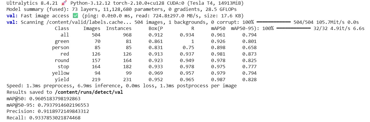
Figure. Validation results of the YOLOv8 model used to detect objects in the Quanser City environment. In the global evaluation, a precision of 0.9119, a recall of 0.9338, an mAP@50 of 0.9605, and an mAP@50-95 of 0.7938 were obtained. These results show that the detector reliably recognizes most of the relevant objects in the scenario and that its performance is sufficiently robust to be integrated into the autonomous driving pipeline.

Figure of training curves

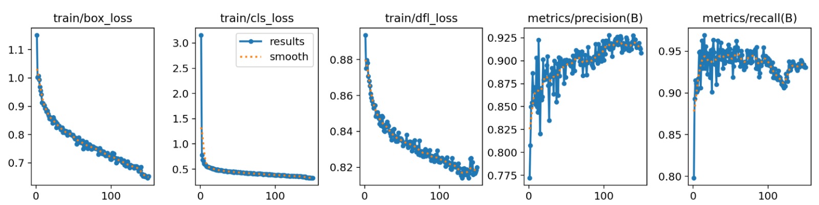
Figure. Evolution of the training losses and the precision and recall metrics during the optimization process. A sustained decrease in the loss functions and a progressive increase in precision and recall can be observed, indicating stable training and adequate convergence of the model.

Figure of validation curves

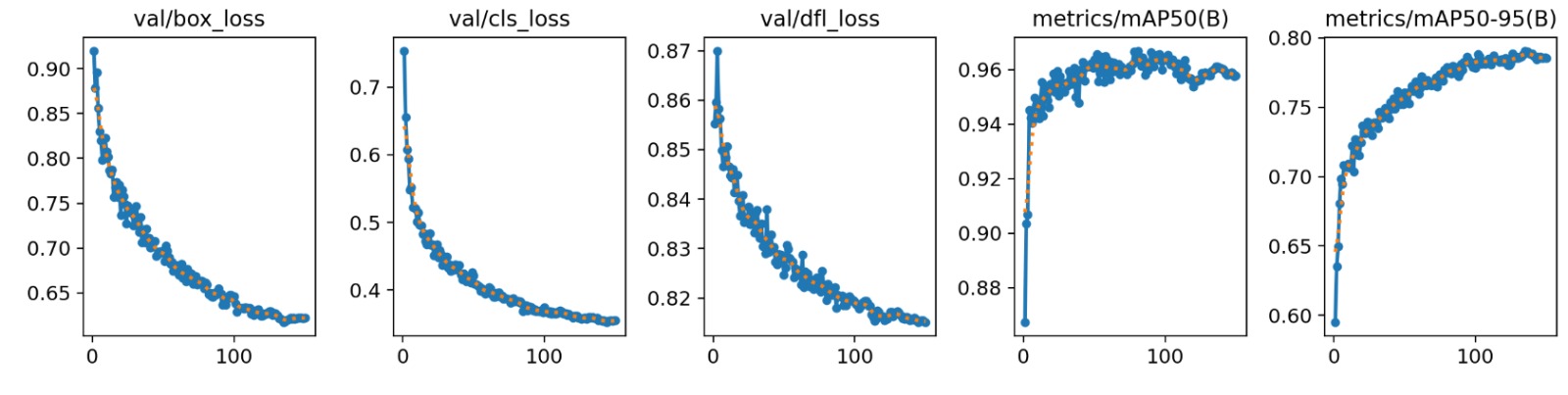
Figure. Evolution of the validation losses and the mAP@50 and mAP@50-95 metrics. The downward trend of the losses and the sustained increase in the performance metrics indicate that the model generalizes properly to unseen data and does not show severe signs of overfitting.

---

Analysis of the trajectory segmentation for turn signal activation

The route generated for the virtual QCar 2 was not only used as a geometric navigation reference, but also as a basis for defining additional road-related behaviors, particularly turn signal activation. To achieve this, after calculating the smoothed global trajectory, the path was segmented in order to identify the specific sections where the left turn signal should be activated and where the right turn signal should be activated. This allowed the vehicle not only to follow a curve, but also to visually express its maneuvers according to more realistic driving rules.

The first trajectory image shows the final global path of the vehicle within the map. In it, the red route can be seen running through the environment delimited by the black dotted outline. This figure validates that the planning algorithm, based on the graph and subsequent smoothing, was able to generate a continuous reference physically consistent with the geometry of the circuit. The trajectory travels through both the outer perimeter and the inner part of the environment, connecting different straight and curved sections smoothly. From a navigation standpoint, this figure represents the nominal path that the vehicle would follow in the absence of events that alter its behavior, such as signs, pedestrians, or obstacles.

Figure of the generated global trajectory

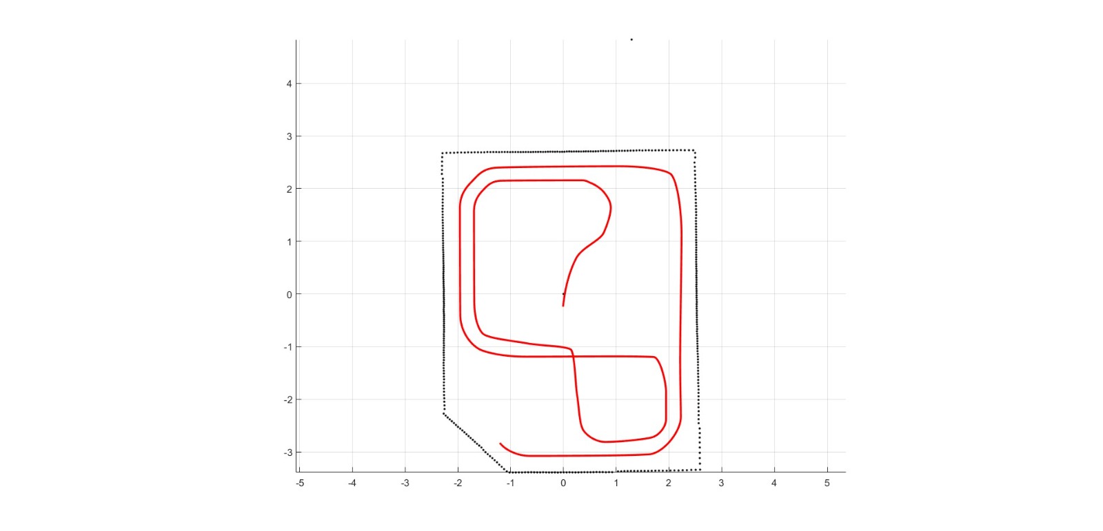
Figure. Final global trajectory of the virtual QCar 2 obtained from the map graph, the shortest-path computation, and smoothing through PCHIP interpolation. The red curve represents the nominal reference that the vehicle will follow within the virtual environment.

The second figure corresponds to the segmentation of that same trajectory for the turn signal logic. In it, the complete route is shown in black, while the sections where the left turn signal should be activated appear in green and the sections where the right turn signal should be activated appear in red. This visualization is especially valuable because it confirms that the rules defined over pairs of nodes were correctly projected onto actual indices of the smoothed trajectory. In other words, the system does not activate the turn signals at a single discrete point, but across continuous intervals of the path, which makes the behavior much more natural and consistent with a real vehicle maneuver.

From an engineering standpoint, this segmentation has a very clear interpretation. The global route is a continuous curve composed of many interpolated points, while the turn signal rules were defined over discrete nodes of the graph. For this reason, it was necessary to construct a mapping between nodes and effective positions within the smoothed trajectory. Once that mapping was established, each relevant transition between nodes could be translated into a specific path segment. The result is precisely the figure shown: a decomposition of the full route into subsets where the lighting logic can operate with temporal and spatial precision.

The figure also makes it possible to visually validate that the important turns of the circuit were classified coherently. The green segments correspond to maneuvers in which the vehicle performs turns or insertions associated with a left turn signal logic, while the red segments represent equivalent maneuvers for the right turn signal. What matters here is not merely that colored segments exist, but that these segments coincide with geometrically congruent areas of the map. In other words, turn signal activation was not arbitrary, but rather consistent with the shape of the trajectory and with the road semantics previously defined through node-to-node rules.

Another important point is that the segmentation does not cover every curve present in the route, but only those transitions that were defined as relevant road maneuvers. This means that the system distinguishes between purely geometric curvature and regulatory turning behavior. This difference is very important in a project like this one, because a smoothed trajectory may contain curvature variations that do not necessarily imply a maneuver that should trigger a turn signal. The implemented logic selects only those sections that correspond to direction changes that are significant from the standpoint of road behavior.

In addition, the use of the auxiliary node located at the center of the intersection made it possible to better model certain complex left turns. Thanks to this, some direction changes that would otherwise appear as an abrupt transition between two extreme nodes could be represented as a more natural arc within the trajectory. In practice, this improves both the geometry of the tracking and the coherence of the interval during which the turn signal is activated. In other words, the auxiliary node improved not only the smoothness of the route, but also the semantic quality of the road-related segmentation.

In validation terms, the turn signal figure demonstrates three important aspects. First, that the mapping between nodes and the interpolated trajectory works correctly. Second, that the rules defined at the topological level are effectively translated into physically located segments where the vehicle executes consistent maneuvers. And third, that the final system can combine geometric navigation with expressive road behavior, which strengthens the presentation of the project as a more complete self-driving architecture.

Figure of turn signal segmentation

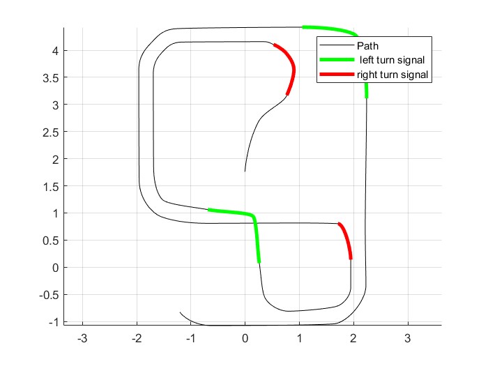
Figure. Segmentation of the trajectory for turn signal activation. The full route is shown in black, the segments where the left turn signal should be activated appear in green, and the segments where the right turn signal should be activated appear in red. This projection validates the correct correspondence between node-to-node rules and real sections of the smoothed trajectory.

Python Inference Process Management via Simulink Callbacks

In order to enable real-time perception, the system relies on an external Python process responsible for running the deep learning inference pipeline. This process is not executed manually, but instead is fully managed from within Simulink through model callbacks.

At the start of the simulation, a Python script is launched using a system-level command executed via PowerShell. The process is started asynchronously, and its process identifier (PID) is retrieved and stored in the MATLAB workspace. This allows the system to keep a reference to the exact instance of the Python process during runtime.

Formally, the initialization step can be described as:

• launching the Python inference server,
• retrieving its PID,
• and storing it for later control.

At the end of the simulation, a termination callback is triggered. In this stage, the stored PID is used to explicitly stop the Python process using a system command. This guarantees that no orphan processes remain running after execution, ensuring proper resource management and avoiding conflicts in subsequent runs.

This mechanism provides a clean and deterministic lifecycle control of the external inference module, enabling seamless integration between Simulink and the Python-based perception system.